<script src="http://me-sitemap.googlecode.com/files/sitemapblog.js" type="text/javascript">
</script>
<script src="http://pengguna-komputer.blogspot.com/feeds/posts/default?max-results=9999&amp;alt=json-in-script&amp;callback=loadtoc">
</script>

PENGOLAHAN CITRA DIGITAL

CELLULAR AUTO MATA

Dewasa ini kebutuhan akan pemahaman terhadap dinamika lahan (land use/ land cover dynamic) semakin tinggi terkait aktivitas manusia di suatu wilayah, seperti dinamika kependudukan, perekonomian, kebencanaan, pertanian maupun kebijakan pemerintah. Interpretasi yang tidak tepat terhadap dinamika lahan mampu menimbulkan dampak negatif di masa yang akan datang. Beberapa alasan tersebut menjadikan kebutuhan pengamatan dan prediksi dinamika spasial lahan menjadi sangat penting. Prediksi perubahan spasial lahan dirasa sangat kompleks dikarenakan banyaknya faktor yang mempengaruhinya, yang menyebabkan perlunya alat untuk melakukannya. Berkat kemajuan teknologi, batasan tersebut mulai dapat diatasi dengan memanfaatkan komputer sebagai alat bantu untuk memprediksi dan melakukan proses iterasi berupa simulasi spasial

“In any type of analysis, it is generally the case that complexity causes greater difficulties in manual methods than in computer methods. Land use forecasting is no exception.” Marshal, N and Lawe, S. (1994). Land use allocation modeling in uni-centric and multi-centric regions. Paper presented at the 1994 TRB National Conference

Cellular Automata (CA) tidak hanya memainkan peran sebagai sebuah kerangka pemodelan spasial melainkan sebuah paradigma untuk berpikir tentang kompleksitas fenomena spasial-temporal. Oleh karena itu, mekanisme CA sangat dibutuhkan tidak hanya dibidang observasi namun lebih kepada bidang perencanaan spasial yang memiliki orientasi masa depan. Selain itu dengan kemampuannya mengakomodasi pendekatan bottom-updan top-down memberikan kreatifitas dalam eksplorasi dimensi ruang spasial.

“Cellular automata is capable of simulating two-dimension state in discrete time, hence it is of spatial-temporal dynamics and the characteristic makes it superior in simulating urban growth and land use change”. Yin C, Yu D, Zhang H, You S, Chen G. (2008). Simulation of urban growth using a cellular automata-based model in a developing nation’s region. Proc. of SPIE Vol. 7143

Salah satu perangkat lunak yang didesain untuk melakukan simulasi dinamika lahan dengan model Cellular Automata adalah LanduseSim. LanduseSim memiliki kemampuan untuk mensimulasikan multi-landuse hingga lebih dari 40 unit lahan yang dapat disimulasikan secara bersamaan. Selain untuk dapat digunakan untuk melakukan simulasi spasial berbasis trend maupun target. Kebebasan dalam melakukan pengaturan terutama untuk perencanaan spasial, simulasi multi-landuse, dan adaptasi scenario planningmenjadi keunggulan LanduseSim dibandingkan aplikasi sejenis.

Beberapa implementasi Pemodelan Dinamika Land Use/Land Cover:

LanduseSim sebagai aplikasi pemodelan dan simulasi spasial perubahan penggunaan lahan berbasis Sistem Informasi Geografis dalam konteks perencanaan wilayah dan kota. Proseding Seminar Nasional CITIES 2014 [Link]

Change to the Land ; Four Scenarios for the Future of the Massachusetts Landscape oleh Harvard University [Link]

Land-Use and Land-Cover Scenarios and Spatial Modeling at the Regional Scale oleh USGS [Link]

Sumber:

http://www.landusesim.com/pelatihan-gis-tingkat-lanjut-landusesim/

PENGOLAHAN CITRA DIGITAL

FOREST FIRE MONITORING

Fire Danger Monitoring and Forecasting

The convergence of plentiful dry wildland fuels and weather favorable for fire ignition and spread signifies high potential for uncharacteristically large and dangerous fires. The ability to characterize the potential for hazardous fire activity requires measurements of fuel condition combined with information from weather forecasts. The availability of long fire histories adds a third dimension, fire probability, which can improve the ability to develop weekly forecasts of the location and number of large fires over a given region (Preisler et. al. 2008).

The USGS uses moderate resolution satellite data to assess live fuel condition for estimating fire danger. Using 23 years of vegetation condition measurements, we are able to determine the relative greenness of current live fuels. High relative greenness values indicate that the vegetation is healthy and vigorous. Low greenness values indicate that the vegetation is under stress, dry (possibly from drought), is behind in annual development, or dead. Forest, shrub, and grassland vegetation with low relative greenness is susceptible to fire ignition during the fire season.

The fire potential index (FPI) integrates weather information from the National Digital Forecast Database and satellite derived vegetation condition information and is used to identify the areas most susceptible to fire ignition (Burgan et.al. 1998). The combination of relative greenness and weather information provides an estimate of the moisture condition of the live and dead vegetation. The FPI is most similar to the Energy Release Component of the National Fire Danger Rating System in that both are moisture-related indexes and neither indicates the effect of wind on fire potential. The FPI indicates the estimated proportion (percentage) of the vegetation that is dry enough to burn, thus the FPI is highest when dead fuel moisture and vegetation greenness are low. The FPI provides local and regional fire planners a quantitative measure of fire ignition risk. Read a description of the current FPI processing flow.

Each day, the U.S. Geological Survey (USGS) in collaboration with the U.S. Forest Service produces 7 day forecasts for all lands. The forecasts are based on historical fire occurrence, current weather and fuels condition. The conditional probability map is an estimate of the likelihood that ignitions will become large fires, given existing levels of the fire danger variables. The large fire forecast map is a probability estimate of the number of fires within a Predictive Service Area exceeding 1000 acres in the forthcoming week. We also produce graphs of total number of expected fires >100 in federal lands per GACC versus day in year.

PENGOLAHAN CITRA DIGITAL

AGRICULTURAL DROUGHT MONITORING AND ASSESMENT

The Famine Early Warning Systems Network (FEWS NET) is a program of the U.S. Agency for International Development (USAID), Office of Food for Peace, that helps target over 1.5 billion dollars of assistance to more than 40 countries each year.  Its history goes back to the mid-1980s, when it had a particular focus on the Sahel, and it continues today with a presence in 17 Sub-Saharan African countries, Haiti, Guatemala, and Afghanistan.  Since its beginning, FEWS NET has been known for its innovative use of geospatial data and satellite remote sensing to help understand what is happening in regions with scarce observations on the ground.  The U.S. Geological Survey, NASA, and NOAA have been developing applications for FEWS NET as long term implementing partners.

In 2011, drought and famine in the Horn of Africa pointed up the vulnerability to climate shocks of people living with poverty, conflict, and weak institutions. This is especially so for herders and subsistence farming livelihoods, which are highly climate-sensitive.  Drought monitoring is as important to famine early warning as tracking market food prices and household nutrition/mortality surveys.  Because station networks in the countries of concern are sparse and often report with significant delay, FEWS NET depends on satellite observations and modeling to fill in the gaps.

Before monitoring crop and rangeland growing conditions, it is necessary to geographically characterize the ways in which households earn income and access food.  FEWS NET does this by producing livelihood zone maps (e.g., http://www.fews.net/docs/Publications/KE_Livelihoods.pdf).  The maps are accompanied by seasonal monitoring calendars, which describe the critical events in the annual cycle of the livelihood systems.  These are essential to understanding the impact of a shock on household income and food access.

Vegetation index imagery is the remote sensing product that has the longest history of use with FEWS NET.  Beginning in the 1980s, NASA provided new images every ten days at a spatial resolution of 8 km to help reveal zones of low plant vigor indicative of drought.  Today, thanks to expedited processing by NASA and USGS, Normalized Difference Vegetation Index (NDVI) images are available every five days at 250 meter resolution, only 12 hours after the last satellite overpass. 

Figure 1 presents an NDVI anomaly image for the Horn of Africa in May, 2011, that clearly illustrates the extent of the devastating failure of rains in the region.

Figure 1.  USGS eMODIS vegetation anomaly image for the Horn of Africa, May 1-10, 2011.

Rainfall is of course a fundamental variable for drought monitoring, and FEWS NET uses Rainfall Estimate (RFE) products from NOAA that blend satellite data with station observations on a 0.1 degree (about 10 km) grid.  These are produced daily by combining cloud top temperature images from geostationary satellites, microwave scattering images from polar orbiting satellites, and rain gauge totals reported to the World Meteorological Organization, where available.  Figure 2 presents an example NOAA RFE image for the African continent.

Figure 2.  Example Rainfall Estimate (RFE) image produced by NOAA for FEWS NET.

In order to better understand the agricultural implications of the RFE, USGS has developed a gridded version of the Water Requirement Satisfaction Index (WRSI), a crop water balance model developed by FAO.  Using grids of potential evapotranspiration computed from output fields of NOAA atmospheric models, along with crop specific coefficients and soil maps, it is possible to compute the extent to which incident rainfall (from RFE) has met the seasonal requirement of staple crops monitored by FEWS NET.  Figure 3 presents an example of output from the WRSI model.

Figure 3.  Example WRSI image for maize in the Horn of Africa in 2009.

A more recent product developed for FEWS NET by USGS uses land surface temperature images, at 1 km resolution, from the NASA MODIS instrument.  These are used in an energy balance calculation to reveal zones of abnormally low crop and rangeland evapotranspiration (ET) due to drought.  Figure 4 presents an example of an ET anomaly (Eta) product.

Figure 4.  Example of an evapotranspiration anomaly image computed from MODIS land

surface temperature data using an energy balance method.  Drought in the Horn of

Africa appears prominently in red tones.

All of these products have their relative strengths and weaknesses.  Fortunately, the underlying geophysical observations behind NDVI, WRSI, and Eta are independent of one another.  This means that they can be used jointly in a convergence of evidence approach to confidently identify zones of drought impact on the landscape.

FEWS NET also uses geospatial climate products that look into the future.  During the 1990s, seasonal forecasts were integrated into preparation of 3-6 month food security outlooks in conjunction with Regional Climate Outlook Forums in Africa.  In the 2000s, the importance of climate change has been recognized through detailed analyses of observed climate trends, diagnostic ocean-atmosphere studies, and interpretations of GCM scenarios.  A series of fact sheets is being produced to present these findings in a way that is helpful to development planners (e.g., http://pubs.usgs.gov/fs/2010/3074/).

The case of the Horn of Africa in 2010-2011 demonstrates how FEWS NET’s understanding of livelihoods and climate (locally and globally) made possible early warning months before the crisis, and enabled pre-positioning of food and supplies in the region (http://www.fews.net/docs/Publications/La_Nina_Brief_East%20Africa_Sept_2... ) In spite of these efforts, conditions overwhelmed the capacity of humanitarian organizations to provide food aid, driving home the lesson that long term disaster reduction lies with political stability, development, and climate change adaptation, rather than emergency response.

In order to support progress in this direction, FEWS NET is applying its experience in drought monitoring to develop loss exceedence curves for crop production shortfall.  Using the RFE record since 2000, a set of 500 seasonal rainfall sequences has been developed statistically to drive the WRSI model.  The 500 WRSI outcomes, in turn can be expressed as yield reductions and shortfall in production on a national scale.  Using these 500 cases of production shortfall, it is possible to build a loss exceedence curve describing the magnitude of agricultural drought impact and associated probability of occurrence.  Figure 5 presents an example of such a curve for national millet harvest production loss in a Sahelian country.  Tools like these will be essential to the implementation of proactive disaster risk reduction programs.  Such programs will be able to greatly reduce human suffering beyond the capabilities of even the best emergency response campaigns.

For more information, please visit

http://www.fews.net

http://earlywarning.usgs.gov/fews

http://www.cpc.ncep.noaa.gov/products/fews/

Figure 5.  Example of a loss exceedence curve for drought impact on the national millet harvest of a Sahelian country.  Work in progress for FEWS NET by H. Jayanthi and G. Husak at the University of California, Santa Barbara.

Sumber:

https://www.agriskmanagementforum.org/content/geospatial-methods-agro-climatic-monitoring-food-security-assessment

PENGOLAHAN CITRA DIGITAL

MAPPING LANDSLIDES TRIGGERED BY THE EARTHQUAKE

The Northridge earthquake provided an unprecedented amount of data for studying the distribution and effects of landslides triggered by an earthquake in an urban area. Detailed field investigations to document earthquake-triggered landslides, which were initiated the day of the earthquake, are continuing. In the first several days following the earthquake, we drove outward from the epicentral area in all directions to locate areas of concentrated landsliding and to find the farthest extent of landsliding, which is defined by small rock and soil falls from very susceptible slopes such as steep road and stream cuts.

High-altitude aerial photography (nominal scale 1:60,000) of the epicentral region was flown by the U.S. Air Force within hours of the earthquake, and we mapped fresh landslides visible on these photos to provide a detailed inventory of ground failures triggered by the earthquake. We mapped more than 11,000 individual landslides on 1:24,000-scale U.S.G.S. topographic base maps. The photos show all but the smallest slope failures and some that were hidden within deep shadows on the north sides of steep slopes.

Landslides as small as 1-2 m across are visible where the slopes were sunlit;where slopes were partly shaded, slides about 5-10 m across are the smallest that could be resolved; thus, the inventory is not complete. However, our field observations indicate that south-facing slopes in most of the landslide area generally are steeper and produced far more landslides than north-facing slopes. Therefore, landslides on north-facing slopes that are not visible on the photos because of shadows probably account for only a small proportion of the total landslides. From our field investigations we estimate that we missed no more than about 20 percent of the landslides that exceeded 5 m in maximum dimension and no more than 50 percent of those smaller than 5 m. In terms of area, however, we estimate that we have mapped more than 90 percent of the area covered by triggered landslides, because most of the landslides that are not visible on the photos are small.

We manually digitized the landslides mapped on the 1:24,000-scale base maps using the Arc/Info geographic information system (GIS). Landslides triggered by the earthquake are plotted as solid polygons on the digital inventory maps (plates 1 and 2). We estimate that location accuracy of landslides mapped from the airphotos to the paper base maps is generally within 10 m and no worse than 20 m. When the paper maps were registered on the digitizer, the computer calculated the root-mean-square (RMS) error in the base-map registration, which averaged 3.6 m and ranged from 0.2 to 10.4 m. Thus, landslide locations plotted on plates 1 and 2 are generally accurate within about 15 m and are no more than 30 m mislocated.

Sumber:

http://pubs.usgs.gov/of/1995/ofr-95-0213/MAPPING.HTML

PENGOLAHAN CITRA DIGITAl

AGRICULTURAL DROUGHT MONITORING AND ASSESMENT

Selain banjir, kekeringan merupakan bencana hidrometeorologis yang juga sering terjadi pada saat

musim kemarau di Indonesia. Beberapa kasus dan kejadian kekeringan di Indonesia lebih banyak

kekeringan agronomis di lahan sawah yang dapat menyebabkan gagal panen. Kebakaran lahan gambut pada saat musim kemarau juga dapat diakibatkan karena kekeringan melanda suatu wilayah. Kekeringan yang lahan dapat terjadi wilayah Nusa Tenggara Timur yang menurut Schidmt-Fergusson memiliki tipe iklim E.

Pemantauan kekeringan dengan data penginderaan jauh sudah banyak dikembangkan. Indek-indek

yang dapat menjadi indikator kekeringan seperti NDVI, SAVI, dan VHI telah dikembangkan untuk

mendeteksi kekeringan suatu vegetasi di suatu wilayah. Selain itu, untuk kekeringan lahan juga telah

dikembangkan dengan memanfaatkan kanal thermal data satelit untuk menghitung fraksi kekeringan

dengan neraca energi.

Aplikasi penginderaan jauh untuk kekeringan lebih banyak menggunakan data resolusi rendah

hingga menengah dan bersifat pemantauan. Data NOAA AVHRR, Terra/Aqua MODIS, dan Data

MTSAT merupakan data yang efektif untuk memantau kekeringan karena memiliki resolusi temporal

yang tinggi. Kekeringan biasanya memiliki luasan yang luas karena terkait dengan klimatologi suatu

wilayah. Skala nasional maupun regional kabupaten sudah baik dilakukan untuk memantau kekeringan

dengan data satelit penginderaan jauh. Error dan uncertainty dari hasil pemantauan dipengaruhi oleh

model atau metode yang digunakan, dan juga resolusi spasial dari citra satelit.

Terdapat beberapa model yang telah dikembangkan adalah model pemantauan kekeringan di lahan

sawah, standardized precipitation index (SPI), dan vegetation health index (VHI). Model digunakan untuk mengetahui tingkat kekeringan di suatu wilayah dengan menggunakan satelit resolusi rendah. Oleh karena itu error dan uncertainty sangat dipengaruhi oleh resolusi spasial selain juga model yang digunakan.

Khusus untuk pemantauan kekeringan lahan sawah error dan uncertainty sangat dipengaruhi oleh peta tematik lahan sawah yang digunakan. 

PENGOLAHAN CITRA DIGITAL

FLOOD DISASTER MANAGEMENT

1. LIST OF ACRONYMS

DEM Digital Elevation Model

DFIRM Digital Flood Insurance Rate Map

DTM Digital Terrain Model

FEMA Federal Emergency Management Agency

FIRM Flood Insurance Rate Map

HEC Hydrologic Engineering Center

NFIP National Flood Insurance Program

TIN Triangular Irregular Network

2. INTRODUCTION

Accurate and current floodplain maps can be the most valuable tools for avoiding severe social and economic losses from floods. Accurately updated floodplain maps also improve public safety. Early identification of flood-prone properties during emergencies allows public safety organizations to establish warning and evacuation priorities. Armed with definitive information, government agencies can initiate corrective and remedial efforts before disaster strikes (Chapman and Canaan, 2001).

GIS is ideally suited for various floodplain management activities such as, base mapping, topographic mapping, and post-disaster verification of mapped floodplain extents and depths. For example, GIS was used to develop a River Management Plan for the Santa Clara River in Southern California. A GIS overlay process was used to further plan efforts and identify conflicting uses along the river and areas for enhancing stakeholder objectives. A 1 inch = 400 ft (1 cm = 122 m) scale base map was created to show topography, planimetric features, and parcels. Attribute data were entered into a separate database and later linked to the appropriate map location. Six layers were created for flood protection related work: 100-year floodplain, 100-year flood way, 25-year interim line, existing facilities, proposed facilities, and flood deposition. The lessons learned from this mapping project indicate that GIS is useful in capturing and communicating a vast amount of information about the study area and the river. While the use of GIS and the process to gather and record data were not without problems, the overall value of GIS was found to overweigh those challenges (Sheydayi, 1999).

3. FLOODPLAIN ANALYSIS STEPS

Typical floodplain analysis involves three major steps (Dodson and Li, 1999):

1. Data collection and preparation

2. Model development and execution

3. Floodplain mapping

GIS can help in all of these steps as described below.

3.1 Data Collection and Assembly

Typical floodplain analysis data requirements include

Topographic Data: stream channel cross-sections and reach lengths

Obstructions Data: bridge and culvert cross-sections

Hydrologic Data: discharge rates for the storm(s) of interest

Hydraulic Data: loss coefficients and hydraulic boundary conditions

These data can be obtained from a variety of sources including the following.

3.1.1 Digital Elevation Data

The latest GIS technology allows the users to draw lines perpendicular to a waterway on a DTM or contour map to extract floodplain cross section data. Using the latest automated floodplain mapping software, DEM, DTM, and TIN data can be used for computing floodplain elevations and mapping floodplain boundaries. TIN data structure has the ability to precisely represent linear (banks, channel bottom, ridges) and point features (hills and sinks), which are critical to accurately define the channel and floodplain geometry. 

In GIS, a line is a series of connected points having a beginning and an end. In ArcInfo, the beginning and end point of each line (arc) is called a "node" and the intermediate points are called vertices. Attributes of each line provide the descriptive information, such as length, direction, and connectivity (Cameron, et al., 1999). GIS has excellent capabilities for storing and manipulating a 3D surface as a DEM, DTM or TIN. GIS can create line features from a TIN of the channel and adjacent floodplain area. These line coverages can be used to create the input data for HEC-RAS.

The U.S. Army Corps of Engineers has developed a new method and incorporated it into an ArcInfo program called CHANNEL to automate the generation of bathymetric (or channel) surfaces along a river reach, requiring only a limited number of channel sections as input. This method is used to develop underwater terrain representation from HEC-2 cross-section input data. The underwater data can be merged with the rest of the terrain representation to form a seamless terrain model that can be directly used for automated geometry extraction for hydraulic models (Long, 1999).

3.1.2 Remote Sensing Data

Although for many legal requirements it is necessary to map flood-prone areas from high-resolution aerial photography, remote sensing data provide initial conditions for flood forecasting, monitoring flooded areas and conducting flood damage assessment. Floodplains have been delineated by using remotely sensed data to infer the extent of the floodplain from vegetation changes, soils, or some other cultural features commonly associated with floodplains (Rango and Anderson, 1974). Low resolution digital Landsat data have been used for producing flood and flood-prone maps at scales of 1:24,000 and 1:62,500 (Sollers et al., 1978). Medium resolution Thematic Mapper (TM) and SPOT satellite data and high resolution IKONOS data can be reasonably expected to produce more accurate delineation of flood prone areas.

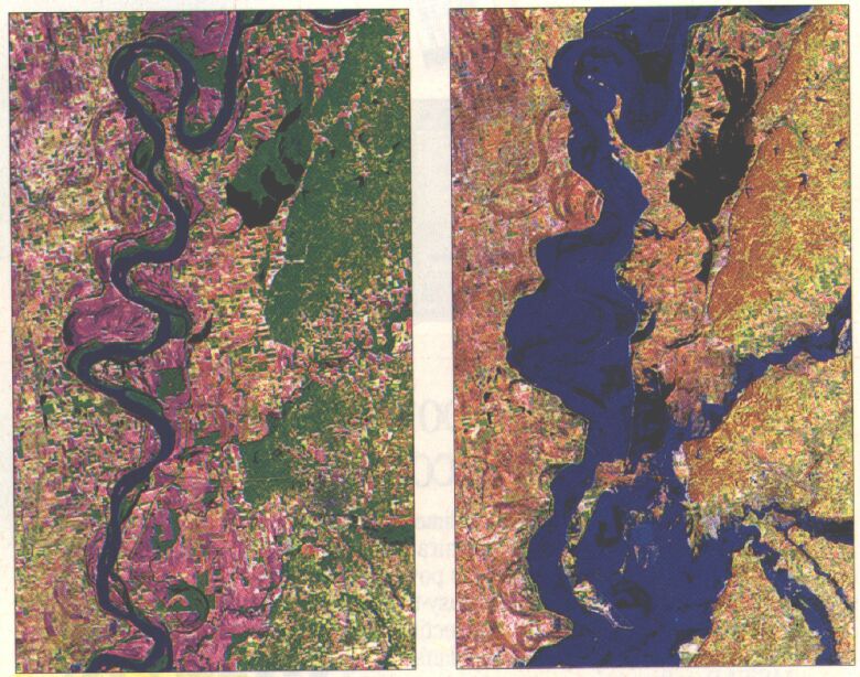
Mississippi River flooding created havoc in the spring of 1997. Figure 1shows 25-meter resolution before and after Landsat images of the flooding. The photos show the Mississippi just below its confluence with the Ohio River in areas south of Cape Girardeau, Missouri. The before flooding image shown at left was taken on July 3, 1996. The post-flooding image shown at right was taken on March 16, 1997. A visual comparison of the two images clearly indicates the extremely large extent of the 1997 flood. Images like this can be effectively used in flood damage assessment and developing flood relief activities (Civil Engineering News, 1997).

Figure 1. Before and After Landsat Imagery for the Mississippi Flood of 1997(Photo Courtesy of Space Imaging EOSAT)

3.2 Model Development And Execution

Floodplain modeling involves two aspects: hydrology and hydraulics (H&H). Hydrologic analysis determines peak flood flows and hydraulic analysis determines peak water surface elevations. A hydrologic model, such HEC-HMS, can be used to model stormwater runoff. This calculation is based on physical characteristics of a drainage area that can be estimated from a GIS database. The runoff information from the hydrologic model can then be combined with stream cross-section information in a hydraulic model, such as HEC-RAS, to determine the depth of flooding.

The integration of a GIS with floodplain computer models allows users to be more productive. Integrated models enable users to devote more time to understanding flooding problems and less time to the mechanical tasks of preparing input data and interpreting the output. 

3.2.1 Three Methods of GIS Linkage

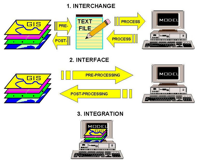
According to a literature review of GIS applications in computer modeling conducted by Heaney et al. (1999) for the U.S. Environmental Protection Agency (EPA), Shamsi (1998, 1999) offers a useful taxonomy to define the different ways a GIS can be linked to computer models. The three methods of GIS linkage defined by Shamsi (2001) illustrated in Figure 2 are: 

1. Interchange method

2. Interface method 

3. Integration method

Figure 2. Three Methods of GIS Linkage

 3.2.1.1 Interchange Method

The interchange method employs a batch processing approach to interchange (transfer) data between a GIS and a computer model. In this method, there is no direct link between the GIS and the model. Both the GIS and the model are run separately and independently. The GIS database is pre-processed to extract model input parameters, which are manually copied into a model input file. Similarly, model output data are manually copied in the GIS to create a new layer for presentation mapping purposes. This is often the easiest method of using a GIS in computer models, and it is the method used most at the present time. Using GIS software to extract floodplain cross-sections from DEM data or runoff curve numbers from land use and soil layers are some examples of the interchange method.

3.2.1.2 Interface Method

The interface method provides a direct link to transfer information between the GIS and the model. The interface method consists of at least the following two components:

A pre-processor, which analyzes and exports the GIS data to create model input files; and

A post-processor, which imports the model output and displays it as a GIS layer. 

The interface method basically automates the data interchange method. The automation is accomplished by adding model-specific menus or buttons to the GIS software interface. The model is executed independently from the GIS; however, the input file is created, at least partially, from within the GIS. The main difference between the interchange and interface methods is the automatic creation of a model input file.

U.S. Army Corps of Engineers HEC-GeoRAS software is a good example of the interface method. Developed as an ArcView GIS extension, GeoRAS allows users to expediently create input data for their HEC-RAS models. Additional GeoRAS information is provided below.

3.2.1.3 Integration Method

GIS integration is a combination of a model and a GIS such that the combined program offers both the GIS and the modeling functions. This method represents the closest relationship between GIS and floodplain models. Two integration approaches are possible:

GIS Based Integration: In this approach, modeling modules are developed in or are called from a GIS. All the four tasks of creating model input, editing data, running the model, and displaying output results are available in GIS. There is no need to exit the GIS to edit the data file or run the model. EPA's BASINS software is a good example of this method.

Model Based Integration: In this method GIS modules are developed in or are called from a computer model. Computation Hydraulics Int.'s (http://www.chi.on.ca/) PCSWMM GIS software is a good example of this method.

Because development and customization tools within most GIS packages provide relatively simple programming capability, the first approach provides limited modeling power. Because it is difficult to program all the GIS functions in a floodplain model, the second approach provides limited GIS capability. Applications are being developed to connect HEC-HMS and HEC-RAS models in a single ArcView GIS environment that would allow users to move easily from a DEM to a floodplain map within a single program (Kopp, 1998).

3.3 Floodplain Mapping

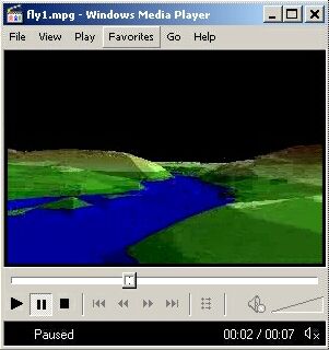
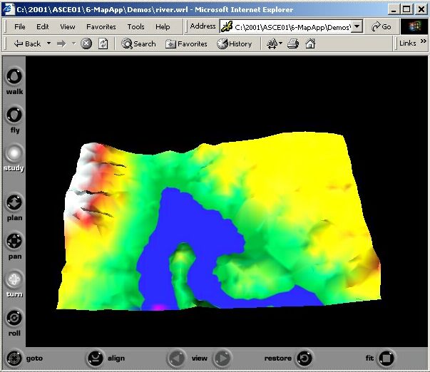
The latest GIS technology allows the users to drape the modeled floodplain boundaries for various design storms on a base map. The modeled inundated areas can be shown as 3D flythrough animations as shown in Figure 3 or in an Internet compatible format for Web browsers as shown in Figure 4.

Figure 3. 3D Flythrough Animation of Modeled Floodplain

Figure 4. Interactive 3D Flythrough Maps of Modeled Floodplain in a Web Browser

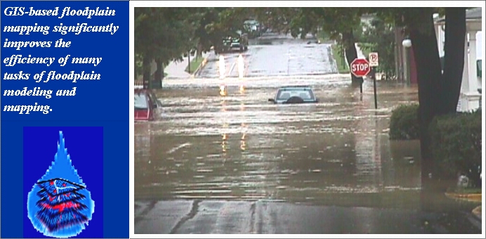
The modeled water surface profiles (elevations) can be imported in a GIS and overlayed upon the terrain surface to create flood maps and determine which areas will be inundated. These maps can be used to develop flood related emergency response procedures. A recent study (Dodson and Li, 1999) compared the results of floodplain mapping for an actual stream channel using the traditional (manual or paper based) and automated (GIS and TIN based) methods. The GIS method used the GIS Stream Pro software described later in this paper. A careful record was maintained of the tasks performed and time required for each task. The results indicated that GIS-based floodplain mapping software provided significant improvements in efficiency for many of the tasks involved in floodplain computations and mapping. Approximately 2/3rd of the effort required to perform a floodplain study was eliminated using the GIS approach. Even more dramatic improvements should be expected when revisions or corrections are required to existing data because recomputing floodplain elevations and remapping floodplain boundaries is fully automated and can be redone almost instantly. 

The study also concluded that the elimination of almost all manual data entry through the use of automated floodplain mapping software should result in significantly fewer human errors in the hydraulic analysis and floodplain mapping procedures. Whereas human errors may be expected 1-10% of all manually computed normal cross-sections (more in longer cross-sections), GIS-based method practically eliminates human errors. Therefore, the floodplain boundaries and profiles produced using the automated procedures should be more accurate under most normal conditions, provided that the TIN model available for use in automated computations is derived from the same topographic data source used for the manual data entry.

Another study conducted in the 3.42 square mile portion of the Mill Creek watershed located in the Lufkin, Texas, indicated that the 100-year floodplain boundaries created using the GIS (Stream Pro) method were different from the effective FIRM boundaries (Kraus, 1999). Some reaches had wider floodplains, while other areas showed distinct reductions in floodplain widths. This study also noted a reduction in time required to manually code the cross-section points into the HEC-RAS model and elimination of human errors due to typographical mistakes. The GIS approach was also found to improve the plotting of floodplains. Before GIS, floodplain plots between cross-sections were subject to interpolation of contours. With GIS, the floodplain is plotted continuously according to the terrain TIN and no interpolation between cross-sections is required.

4. SOFTWARE EXAMPLES

Some floodplain mapping and modeling software examples are presented below.

4.1 DHI MIKE Products

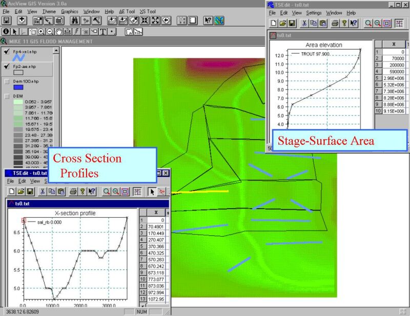
DHI Inc. (http://www.dhi.dk) has three floodplain modeling packages that have GIS linkage capabilities: MIKE 11, MIKE 21, and MIKE FLOOD. MIKE 11 models floodplain hydraulics. MIKE 11 GIS is a spatial decision support system for river and floodplain management. It is an ArcView GIS extension for Mike 11 models. The 2001 release of MIKE 11 includes a new floodplain encroachment model to assess the hydrodynamic impacts of floodplain encroachments on the water and energy levels. Figure 5 shows a MIKE 11 GIS screenshot illustrating how a DEM grid can be used in ArcView to create floodplain cross-sections for input to program's hydraulic engine. Today, many flood studies require detailed spatial resolution which can be achieved through the application of 2D techniques. MIKE 21 is DHI's preferred 2D engineering modeling tool for rivers, estuaries and coastal waters. DHI's latest floodplain modeling package, MIKE FLOOD combines the best features of 1D and 2D flood modeling technology. MIKE FLOOD is assembled from the components taken from MIKE 11 and MIKE 21. This combination allows users to model some areas in 2D detail, while other areas can be modeled in 1D. Like MIKE 11 and MIKE 21, MIKE FLOOD also has GIS linkage capabilities which can be used, for example, to produce inundation maps as a result of levee or embankment failures. 

4.2 HEC-GeoRAS

The HEC-RAS system is intended for calculating water surface profiles in a full network of channels, a dendritic system, or a single river reach. HEC-GeoRAS for ArcView is an ArcView GIS extension specifically designed to process geospatial data for use with HEC-RAS. The extension allows users to create an HEC-RAS import file containing geometric attribute data from an existing DTM and complementary data sets. GeoRAS automates the extraction of spatial parameters for HEC-RAS input, primarily the 3D stream network and the 3D cross-section definition. Results exported from HEC-RAS may also be processed in GeoRAS. ArcView 3D Analyst extension is required to use GeoRAS. Spatial Analyst is recommended. 

Free download of GeoRAS program is available from the HEC software website http://www.hec.usace.army.mil/software/. While the GeoRAS program was developed for HEC-RAS; it is not exclusive to HEC-RAS. It can be applied in the floodplain analysis and modeling using other river analysis programs. An ArcInfo version of GeoRAS is also available. To use this version, a knowledge of ArcInfo, ARCEDIT, and ARCPLOT is advantageous, but not necessary. 

4.2.1 Inundation Mapping

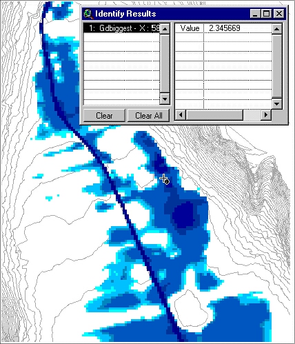
HEC-RAS modeling results are exported to a data exchange text file that includes the locations of the cross-section cut lines along with water surface profile data and a set of polygons that describe the extent of the modeled floodplain. A line coverage of cross-section cut lines is created and attributed with water surface elevations. For inundation mapping, a TIN of the water surface is then generated from the water surface elevations. Background coverages may be displayed along with the inundation data to determine flood prone areas. Figure 6 shows an example inundation map created by GeoRAS. It shows a flooding depth grid with ArcView's Identify Results window for water depth. Deeper water is indicated by darker blue color.

Figure 5. Mike 11 Screenshot Showing How to Draw Lines on a DEM Grid to Generate Floodplain Cross-Sections for Model Input

4.3 ArcGIS Hydro Data Model

Esri's ArcGIS Hydro Data Model

(http://www.Esri.com/software/arcgisdatamodels/arcgishydromodel/index.html) can be updated to display purely cartographic data, such as the types of data used in creating NFIP floodplain maps. A typical geodatabase model for floodplain mapping may include the following data:

Benchmark feature class: A benchmark elevation point depicted on the existing FIRM

Bridges, buildings, and docks classes: Polygons outlining their respective features

Corporate limits and extraterritorial jurisdictional (ETJ) classes: Line features delineating city limits and ETJ areas

Parcels feature class: polygons and attribute information of each parcel along the river

Contours and spot elevations: Elevation information used to develop the floodplains

Floodplain class: Flood hazards shown on DFIRM, including the 100- and 500-year floodplains

Waterbodies and roads annotation: Labels for these features

This geodatabase includes more information than the required data for a standard DFIRM database. However, a DFIRM database may contain much more information than listed here. The parcels, buildings, and spot elevations classes are all examples of data that are neither required in DFIRM database nor shown on the floodplain maps, but can provide useful information. 

Figure 6. Inundation Map Created by HEC-GeoRAS

4.4 GIS Stream Pro

Many utility programs are available to create the input data for floodplain models. These programs use an approach similar to the interchange GIS linkage method described above. For example, GIS Stream Pro from Dodson & Associates (http://www.dodson-hydro.com) is an ArcView Extension that runs with ArcView 3D Analyst Extension. It simplifies HEC-RAS input by extracting 3D stream network and the 3D cross-section data from a terrain TIN and automates floodplain delineation based on the HEC-RAS Geographic Data Export File and the original terrain TIN used to create the geometry import file. It uses 3D spatial features to identify the stream network and HEC-RAS model layout. Once identified, GIS Stream Pro generates the HEC-RAS Geometry Import File. GIS Stream Pro imports terrain data in ArcInfo format from various data sources, such as, DEM, DTM, field survey, and LIDAR. It can define base 2D spatial features, such as, stream centerline, left and right bank lines, center of flow paths for the channel and overbanks, and cross-section layouts as ArcView shapes over the terrain TIN. Attributed 3D spatial data for 3D stream centerlines and 3D cross-sections can also be generated.

4.5 RiverCAD

RiverCAD is a floodplain mapping software from Boss International (http://www.bossintl.com). RiverCAD uses its own built-in AutoCAD compatible CAD system which allows creation of 3D CAD drawings of HEC-RAS (or HEC-2) models. It displays HEC-RAS results directly on top of a contour map, showing the extent of water surface with regard to the ground topography. Reportedly, RiverCAD also creates scaled cross-section and profile plots that are ready for FEMA submittal. It will read and display FEMA Q3 floodplain maps, and can generate ArcView GIS shapefiles of HEC-RAS input data and analysis results. It allows creation of cross-section data from a contour map, TIN, or DTM by simply drawing a line. It can directly read survey files, USGS DEM files, and ArcInfo GIS files.

5. CASE STUDY

Many communities are using the latest Information Technology (IT) tools to develop "Watershed Information Systems." For example, the City of Charlotte and Mecklenburg County of North Carolina, which are one of the fastest growing metropolitan areas of the United States have developed a watershed information system called WISE that integrates data management, GIS, and standard stormwater analysis programs like HEC-1, HEC-2, HEC-HMS, and HEC-RAS. Using this method, the existing H&H models can be updated at a fraction (less than $100,000) of the cost of developing a new model (more than $1 million). WISE data management system emphasizes data storage and access using pre- and post-processing techniques. Pre-processors funnel appropriate data in the correct format to industry standard H&H models. Post-processors extract and assimilate model results inside a GIS. WISE consists of several modules. The terrain module of WISE effectively manages large amounts of digital terrain data and can merge terrain data from various sources into a single, seamless terrain model. This module creates TINS and raster grids for use in other WISE modules. The hydrology module uses data from previously existing models, GIS coverages, and surveys to generate hydrologic data sets, including curve numbers, time of concentrations, and hydrographs. The hydraulic module generates working hydraulic models, flood profiles, floodplain mapping, and hydraulic results from WISE data sets such as total stations or GPS data survey data and digital terrain data (Edelman et al., 2001). The basic model data consist of elevation contours and H&H factors, such as the rainfall, soil characteristics, slope contours, creek characteristics (size, shape, and roughness), physical features (culverts and bridges) and past, current, and anticipated land use information. 

Hurricane Floyd was probably the most powerful hurricane in the Atlantic Basin since Hurricane Andrew. It was definitely the most intense of the 1999 Atlantic Basin Hurricanes when its winds reached 155 mph. It started out as a depression in the Central Atlantic on September 7, 1999. Severe riverine flooding occurred in Eastern North Carolina due to heavy rainfall associated with Hurricane Floyd, causing an $800 million damage to property. This extensive damage required more than $100 million in post-disaster mitigation funding from the government. Because detailed flood data were not available for specific waterways, FEMA and North Carolina Department of Emergency Management requested that hydraulic studies be performed to establish approximate base flood (100-year) elevations to assist in proper floodplain management. Flood Hazard Mitigation Plans were prepared for the four major watersheds located in the central portion of Mecklenburg County. Extensive GIS data were utilized to perform the hazard evaluation and risk assessment including past flooding complaints tracked by the City of Charlotte and Meclkelnburg County, flood insurance policy and claim data, GPS elevations and locations of floodprone structures. Remarkably, there were more than 2,500 structures in the 100-year floodplain. A GIS layer of the existing floodplain and floodway boundaries was created to facilitate the flood hazard evaluation. 

6. USEFUL WEB SITES

ArcGIS Hydro Data Model -

http://www.Esri.com/software/arcgisdatamodels/arcgishydromodel/index.html

DHI's Mike 11, Mike 21, and Mike-Flood - http://www.dhi.dk

FEMA - http://www.fema.gov/

GIS Stream Pro Software - http://www.dodson-hydro.com

HEC-GeoRAS Software - http://www.hec.usace.army.mil/software/

NFIP - http://www.fema.gov/nfip

RiverCAD Software http://www.bossintl.com/

Sumber:

http://proceedings.esri.com/library/userconf/proc02/pap0490/p0490.htm